Supervised Learning(Part-7)
Random Forest
The Random Forest Classifier
Random forest, like its name implies, consists of a large number of individual decision trees that operate as an ensemble. Each individual tree in the random forest spits out a class prediction and the class with the most votes becomes our model’s prediction (see figure below).

Visualization of a Random Forest Model Making a Prediction
The fundamental concept behind random forest is a simple but powerful one — the wisdom of crowds. In data science speak, the reason that the random forest model works so well is:
A large number of relatively uncorrelated models (trees) operating as a committee will outperform any of the individual constituent models.
The low correlation between models is the key. Just like how investments with low correlations (like stocks and bonds) come together to form a portfolio that is greater than the sum of its parts, uncorrelated models can produce ensemble predictions that are more accurate than any of the individual predictions. The reason for this wonderful effect is that the trees protect each other from their individual errors (as long as they don’t constantly all err in the same direction). While some trees may be wrong, many other trees will be right, so as a group the trees are able to move in the correct direction. So the prerequisites for random forest to perform well are:
There needs to be some actual signal in our features so that models built using those features do better than random guessing.
The predictions (and therefore the errors) made by the individual trees need to have low correlations with each other.
An Example of Why Uncorrelated Outcomes are So Great
The wonderful effects of having many uncorrelated models is such a critical concept that I want to show you an example to help it really sink in. Imagine that we are playing the following game:
I use a uniformly distributed random number generator to produce a number.
If the number I generate is greater than or equal to 40, you win (so you have a 60% chance of victory) and I pay you some money. If it is below 40, I win and you pay me the same amount.
Now I offer you the the following choices. We can either:
Game 1 — play 100 times, betting $1 each time.
Game 2— play 10 times, betting $10 each time.
Game 3— play one time, betting $100.
Which would you pick? The expected value of each game is the same:
Expected Value Game 1 = (0.60*1 + 0.40*-1)*100 = 20
Expected Value Game 2= (0.60*10 + 0.40*-10)*10 = 20
Expected Value Game 3= 0.60*100 + 0.40*-100 = 20
Outcome Distribution of 10,000 Simulations for each Game
What about the distributions? Let’s visualize the results with a Monte Carlo simulation (we will run 10,000 simulations of each game type; for example, we will simulate 10,000 times the 100 plays of Game 1). Take a look at the chart on the left — now which game would you pick? Even though the expected values are the same, the outcome distributions are vastly different going from positive and narrow (blue) to binary (pink).
Game 1 (where we play 100 times) offers up the best chance of making some money — out of the 10,000 simulations that I ran, you make money in 97% of them! For Game 2 (where we play 10 times) you make money in 63% of the simulations, a drastic decline (and a drastic increase in your probability of losing money). And Game 3 that we only play once, you make money in 60% of the simulations, as expected.
Probability of Making Money for Each Game
So even though the games share the same expected value, their outcome distributions are completely different. The more we split up our $100 bet into different plays, the more confident we can be that we will make money. As mentioned previously, this works because each play is independent of the other ones.
Random forest is the same — each tree is like one play in our game earlier. We just saw how our chances of making money increased the more times we played. Similarly, with a random forest model, our chances of making correct predictions increase with the number of uncorrelated trees in our model.
Ensuring that the Models Diversify Each Other
So how does random forest ensure that the behavior of each individual tree is not too correlated with the behavior of any of the other trees in the model? It uses the following two methods:
Bagging (Bootstrap Aggregation) — Decisions trees are very sensitive to the data they are trained on — small changes to the training set can result in significantly different tree structures. Random forest takes advantage of this by allowing each individual tree to randomly sample from the dataset with replacement, resulting in different trees. This process is known as bagging.
Notice that with bagging we are not subsetting the training data into smaller chunks and training each tree on a different chunk. Rather, if we have a sample of size N, we are still feeding each tree a training set of size N (unless specified otherwise). But instead of the original training data, we take a random sample of size N with replacement. For example, if our training data was [1, 2, 3, 4, 5, 6] then we might give one of our trees the following list [1, 2, 2, 3, 6, 6]. Notice that both lists are of length six and that “2” and “6” are both repeated in the randomly selected training data we give to our tree (because we sample with replacement).
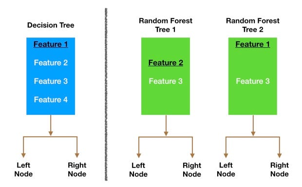
Node splitting in a random forest model is based on a random subset of features for each tree.
Feature Randomness — In a normal decision tree, when it is time to split a node, we consider every possible feature and pick the one that produces the most separation between the observations in the left node vs. those in the right node. In contrast, each tree in a random forest can pick only from a random subset of features. This forces even more variation amongst the trees in the model and ultimately results in lower correlation across trees and more diversification.
Let’s go through a visual example — in the picture above, the traditional decision tree (in blue) can select from all four features when deciding how to split the node. It decides to go with Feature 1 (black and underlined) as it splits the data into groups that are as separated as possible.
Now let’s take a look at our random forest. We will just examine two of the forest’s trees in this example. When we check out random forest Tree 1, we find that it it can only consider Features 2 and 3 (selected randomly) for its node splitting decision. We know from our traditional decision tree (in blue) that Feature 1 is the best feature for splitting, but Tree 1 cannot see Feature 1 so it is forced to go with Feature 2 (black and underlined). Tree 2, on the other hand, can only see Features 1 and 3 so it is able to pick Feature 1.
So in our random forest, we end up with trees that are not only trained on different sets of data (thanks to bagging) but also use different features to make decisions.
And that, my dear reader, creates uncorrelated trees that buffer and protect each other from their errors.
Conclusion
Random forests are a personal favorite of mine. Coming from the world of finance and investments, the holy grail was always to build a bunch of uncorrelated models, each with a positive expected return, and then put them together in a portfolio to earn massive alpha (alpha = market beating returns). Much easier said than done!
Random forest is the data science equivalent of that. Let’s review one last time. What’s a random forest classifier?
The random forest is a classification algorithm consisting of many decisions trees. It uses bagging and feature randomness when building each individual tree to try to create an uncorrelated forest of trees whose prediction by committee is more accurate than that of any individual tree.
What do we need in order for our random forest to make accurate class predictions?
We need features that have at least some predictive power. After all, if we put garbage in then we will get garbage out.
The trees of the forest and more importantly their predictions need to be uncorrelated (or at least have low correlations with each other). While the algorithm itself via feature randomness tries to engineer these low correlations for us, the features we select and the hyper-parameters we choose will impact the ultimate correlations as well.


Comments
Post a Comment